Our objective is to synthesize a random field model for coherent fields. We've already discussed how ignoring deformations effects the mean and covariance of random coherent fields. Assuming the spatial process is Gauss-Markov, then where one would expect to see random realizations from a KL expansion (say from training data) to produce coherent signals,  the leading EOF (POD) modes are such that alas this is not what happens. As the spectrum is truncated, coherence is lost, even if the deformation was a mere translation of an otherwise static field.

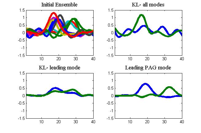
Here, produce a new coherent random field model by constructing principal coherent features and the principal appearance and geometry modes (PAG modes). As the results show (see above), even one leading mode of the PAG-expansion produces coherent random realizations. This is because we extract both the amplitude (appearance) and deformation (geometry) modes from the data. This approach also leads to a variety of interesting representations including what we have termed Deformable-ROM. A particular example, Deformable-POD is discussed elsewhere and leads to very robust techniques for reduced order modeling complimenting the data-driven scale-cascaded model for tracking discussed earlier. We visit deformable-rom later, here  we summarize the basic mechanics of calculating the principal appearance and geometry modes, and realizing coherent random fields.

We define a deformation of a coherent field as:

,

where q is the deformation of the field X.  Modeling these as Gauss-Markov processes, we construct the KL-expansion:

Thus, for random vectors, and corresponding bases U_q and U_x so that the random field consists of an amplitude and position part:

This can be expressed in a number of ways:

Equivalently,

Here,  X o q, is the coherent random field. U_x and U_q are the principal appearance and geometry modes respectively, and U_x are the principal coherent features. The label (3) is the expansion of the random fields in terms of the principal appearance and geometry modes, with a mean deformation and random perturbation (2), and  (1) is the deformable reduced order model.

How is a random field estimated from ensemble (or snapshot) data? Here are the steps:

1. Coalesce the ensemble and extract the mean deformation, mean appearance, and deformation ensemble perturbations and field appearance perturbations.
2. From the deformation ensemble of perturbations, calculate the geometry modes U_q and spectrum S_q
3. From the deviations of coalesced ensemble from the coalesced mean, calculate U_x and spectrum S_x

The result of doing this and comparing it with the standard is shown in the figure at the begining of this entry. Whether one uses all the modes in the KL expansion of the original data, or the leading mode, coherence is not preserved. On the other hand, because of the dominant motion, the leading PAG mode is enough to produce perfect random realizations. We want to point out that some of the ensemble members could be "observations", possibly sparse, possibly noisy. In the examples shown here, only every third grid value is used for coalescence and the signals themselves are noisy, accomodating for this fact.

A key question is how are we supposed to measure what perfect synthesis is? One way to do this is to extract features from the data. The peak values, number of peaks, the signal variance (scale), or the entropy and compare that between the provided data and the realized data. We will also discuss this shortly.